Data Loading
import pandas as pd
import matplotlib.pyplot as plt
import matplotlib.ticker as ticker
import numpy as np
import seaborn as sns
import pymc as pm
import bambi as bmb
import arviz as az
import statsmodels.api as sm
from sklearn.preprocessing import OneHotEncoder
EPA EGRID: https://
eGRID Demographic Data
egrid_demo = pd.read_csv("data/egrid2023_demo.csv")[1:]
egrid_demo_multiindex = pd.read_csv("data/egrid2023_demo.csv", header = [0,1])
egrid_demo
/tmp/ipykernel_1504/2054141767.py:1: DtypeWarning: Columns (0,1,4,5,6,9,12,13,14,15,16,17,18,19,20,21,22,23,24,25,26,27,28,29,30,31,32,33,34,35,36,37,38,39,40,41,42,43,44,45,46,47,48,49,50,51,52,53,54,55,56,57,58,59,60,61,62,63,64) have mixed types. Specify dtype option on import or set low_memory=False.
egrid_demo = pd.read_csv("data/egrid2023_demo.csv")[1:]
egrid_plant = pd.read_csv("data/egrid2023_plant.csv")[1:]
egrid_plant
/tmp/ipykernel_1504/1590308207.py:1: DtypeWarning: Columns (0,1,4,6,8,16,17,19,20,22,23,27,29,33,34,35,50,51,52,53,55,56,58,59,60,61,62,63,64,65,66,67,68,69,71,72,74,82,85,86,97,98,99,102,107,122) have mixed types. Specify dtype option on import or set low_memory=False.
egrid_plant = pd.read_csv("data/egrid2023_plant.csv")[1:]
egrid_joined = pd.merge(egrid_plant, egrid_demo, on="DOE/EIA ORIS plant or facility code")
egrid_joined.head()Cleaning eGRID data
#Extract county FIPS from egrid data

#relevant_columns = ['Plant primary fuel category_x', 'Plant annual net generation (MWh)', 'Total Population', 'People of Color (%)', 'Low Income (%)', 'Less Than High School Education (%)', 'Limited English Speaking (%)', 'Unemployment Rate (%)', 'Limited Life Expectancy (%)', 'Demographic Index', "National Percentile of Over Age 64"]

#rename after merge
egrid_joined['Plant state abbreviation'] = egrid_joined['Plant state abbreviation_x']
egrid_joined['Plant latitude'] = egrid_joined['Plant latitude_x']
egrid_joined['Plant longitude'] = egrid_joined['Plant longitude_x']

# dropna for any relevant column
num_blocks_dropped = egrid_joined[['Plant FIPS state code', 'Plant FIPS county code','Plant state abbreviation','Plant county name', 'Plant latitude', 'Plant longitude', 'Total Population', 'People of Color (%)', 'Low Income (%)', 'Less Than High School Education (%)', 'Limited English Speaking (%)', 'Unemployment Rate (%)', 'Limited Life Expectancy (%)', 'Under Age 5 (%)', 'Over Age 64 (%)']].isnull().any(axis=1).sum()
egrid_dropped = egrid_joined.dropna(subset=['Plant FIPS state code', 'Plant FIPS county code','Plant state abbreviation','Plant county name', 'Plant latitude', 'Plant longitude', 'Total Population', 'People of Color (%)', 'Low Income (%)', 'Less Than High School Education (%)', 'Limited English Speaking (%)', 'Unemployment Rate (%)', 'Limited Life Expectancy (%)', 'Under Age 5 (%)', 'Over Age 64 (%)'])
#egrid_dropped['Plant FIPS state code str'] = egrid_dropped['Plant FIPS state code'].astype(int).astype(str)

#force the FIPS state code to numeric, make it an integer (some were floating point) fill it to the default 2 spaces (e.g 8 become 08)
egrid_dropped['Plant FIPS state code'] = pd.to_numeric(egrid_dropped['Plant FIPS state code'], errors='coerce')
egrid_dropped['Plant FIPS state code'] = egrid_dropped['Plant FIPS state code'].astype(int).astype(str).str.zfill(2)

#force the FIPS county code to numeric, fill it to the default 3 spaces (e.g 1 become 001)
egrid_dropped['Plant FIPS county code'] = pd.to_numeric(egrid_dropped['Plant FIPS county code'], errors='coerce')
egrid_dropped['Plant FIPS county code'] = egrid_dropped['Plant FIPS county code'].astype(int).astype(str).str.zfill(3)  #county, state codes sometimes int or decimal

# concatenate State and County FIPS for unique ID
egrid_dropped['County FIPS'] = egrid_dropped['Plant FIPS state code'] + egrid_dropped['Plant FIPS county code']

# assign plant counties to treatment group
egrid_dropped['has_plant'] = 1

# relevant columns for multiple hypothesis testing
columns_select = ['County FIPS', 'Plant county name', 'Plant state abbreviation','Plant latitude', 'Plant longitude', 'has_plant', 'Total Population', 'People of Color (%)', 'Low Income (%)', 'Less Than High School Education (%)', 'Limited English Speaking (%)', 'Unemployment Rate (%)', 'Limited Life Expectancy (%)', "Plant primary fuel category_x", "Plant annual net generation (MWh)", 'Over Age 64 (%)', 'Under Age 5 (%)']
egridf = egrid_dropped[columns_select]

# clean columns used for analysis that have odd formatting and discrepancies
clean_me = ['Total Population', 'People of Color (%)', 'Low Income (%)', 'Less Than High School Education (%)', 'Limited English Speaking (%)', 'Unemployment Rate (%)', 'Limited Life Expectancy (%)', 'Over Age 64 (%)', 'Under Age 5 (%)']
for col in clean_me:
    cleaned = egrid_dropped[col].astype(str).str.replace(r'[,\(\)]', '', regex=True)
    egridf[col] = pd.to_numeric(cleaned, errors='coerce')
    num_blocks_dropped += egridf.isnull().any(axis=1).sum()
    egridf = egridf.dropna()
    egridf[col] = egridf[col].astype(int)

num_blocks_dropped += egridf.isnull().any(axis=1).sum()
egridf.dropna()
print(f'Number of plant communities dropped in processing: {num_blocks_dropped} with 7756 remaining (about 9% loss)')
egridf.shape
Number of plant communities dropped in processing: 760 with 7756 remaining (about 9% loss)
/tmp/ipykernel_1504/2527193710.py:16: SettingWithCopyWarning:
A value is trying to be set on a copy of a slice from a DataFrame.
Try using .loc[row_indexer,col_indexer] = value instead

See the caveats in the documentation: https://pandas.pydata.org/pandas-docs/stable/user_guide/indexing.html#returning-a-view-versus-a-copy
  egrid_dropped['Plant FIPS state code'] = pd.to_numeric(egrid_dropped['Plant FIPS state code'], errors='coerce')
/tmp/ipykernel_1504/2527193710.py:17: SettingWithCopyWarning:
A value is trying to be set on a copy of a slice from a DataFrame.
Try using .loc[row_indexer,col_indexer] = value instead

See the caveats in the documentation: https://pandas.pydata.org/pandas-docs/stable/user_guide/indexing.html#returning-a-view-versus-a-copy
  egrid_dropped['Plant FIPS state code'] = egrid_dropped['Plant FIPS state code'].astype(int).astype(str).str.zfill(2)
/tmp/ipykernel_1504/2527193710.py:20: SettingWithCopyWarning:
A value is trying to be set on a copy of a slice from a DataFrame.
Try using .loc[row_indexer,col_indexer] = value instead

See the caveats in the documentation: https://pandas.pydata.org/pandas-docs/stable/user_guide/indexing.html#returning-a-view-versus-a-copy
  egrid_dropped['Plant FIPS county code'] = pd.to_numeric(egrid_dropped['Plant FIPS county code'], errors='coerce')
/tmp/ipykernel_1504/2527193710.py:21: SettingWithCopyWarning:
A value is trying to be set on a copy of a slice from a DataFrame.
Try using .loc[row_indexer,col_indexer] = value instead

See the caveats in the documentation: https://pandas.pydata.org/pandas-docs/stable/user_guide/indexing.html#returning-a-view-versus-a-copy
  egrid_dropped['Plant FIPS county code'] = egrid_dropped['Plant FIPS county code'].astype(int).astype(str).str.zfill(3)  #county, state codes sometimes int or decimal
/tmp/ipykernel_1504/2527193710.py:24: SettingWithCopyWarning:
A value is trying to be set on a copy of a slice from a DataFrame.
Try using .loc[row_indexer,col_indexer] = value instead

See the caveats in the documentation: https://pandas.pydata.org/pandas-docs/stable/user_guide/indexing.html#returning-a-view-versus-a-copy
  egrid_dropped['County FIPS'] = egrid_dropped['Plant FIPS state code'] + egrid_dropped['Plant FIPS county code']
/tmp/ipykernel_1504/2527193710.py:27: SettingWithCopyWarning:
A value is trying to be set on a copy of a slice from a DataFrame.
Try using .loc[row_indexer,col_indexer] = value instead

See the caveats in the documentation: https://pandas.pydata.org/pandas-docs/stable/user_guide/indexing.html#returning-a-view-versus-a-copy
  egrid_dropped['has_plant'] = 1
/tmp/ipykernel_1504/2527193710.py:37: SettingWithCopyWarning:
A value is trying to be set on a copy of a slice from a DataFrame.
Try using .loc[row_indexer,col_indexer] = value instead

See the caveats in the documentation: https://pandas.pydata.org/pandas-docs/stable/user_guide/indexing.html#returning-a-view-versus-a-copy
  egridf[col] = pd.to_numeric(cleaned, errors='coerce')
(7756, 17)# add regions to egridf for regional exploration based on EPA regional categorization
epa_regions_by_state = {
'CT': 1, 'ME': 1, 'MA': 1, 'NH': 1, 'RI': 1, 'VT': 1,
'NJ': 2, 'NY': 2, 'PR': 2, 'VI': 2,
'DE': 3, 'DC': 3, 'MD': 3, 'PA': 3, 'VA': 3, 'WV': 3,
'AL': 4, 'FL': 4, 'GA': 4, 'KY': 4, 'MS': 4, 'NC': 4, 'SC': 4, 'TN': 4,
'IL': 5, 'IN': 5, 'MI': 5, 'MN': 5, 'OH': 5, 'WI': 5,
'AR': 6, 'LA': 6, 'NM': 6, 'OK': 6, 'TX': 6,
'IA': 7, 'KS': 7, 'MO': 7, 'NE': 7,
'CO': 8, 'MT': 8, 'ND': 8, 'SD': 8, 'UT': 8, 'WY': 8,
'AZ': 9, 'CA': 9, 'HI': 9, 'NV': 9, 'AS': 9, 'GU': 9, 'MP': 9, 'FM': 9, 'MH': 9, 'PW': 9,
'AK': 10, 'ID': 10, 'OR': 10, 'WA': 10
}
egridf['EPA Region'] = egridf['Plant state abbreviation'].map(epa_regions_by_state)plant_per_county = egridf.groupby("County FIPS").size()
plant_per_county_plusone = plant_per_county[plant_per_county > 1]
print(f'There are {plant_per_county_plusone.size} counties with more than one utility plant')There are 1005 counties with more than one utility plant
egridf.to_csv('data/egrid_counties.csv')It’s important to note that there are only 1422 unique counties, but over 7,000 plants. Thats because the plant is pulling the information of a 3 mile radius around it, and there may be multiple plants in one county. One reason that could be for this is one county having multiple different types of plants. Lets see below:
Data Processing for Non-Host Communities
Notes about EJSCREEN Data:
Data obtained here: https://
egrid details here: https://
ejscreen in action here: https://
ejscreen documentation here: https://
other resource i couldnt figure out: https://
ejscreen tool archive: https://
First, get latitude and longitude for each block group and convert to radians to efficiently calculate block groups distance to a utility plant
import requests
# ref https://www.geeksforgeeks.org/python/how-to-download-files-from-urls-with-python/#

#This is census data for each block group id, it gives the mean latitude and longitude
url = 'https://www2.census.gov/geo/docs/reference/cenpop2020/blkgrp/CenPop2020_Mean_BG.txt'

response = requests.get(url)
file_path = 'data/CenPop2020_Mean_BG.txt'

if response.status_code == 200:
    with open(file_path, 'wb') as file:
        file.write(response.content)
    print('File downloaded successfully')
else:
    print('Failed to download file')
File downloaded successfully
#block group means
mean_bg = pd.read_csv(file_path)

mean_bg['STATEFP'] = mean_bg['STATEFP'].astype(str).str.zfill(2)
mean_bg['COUNTYFP'] = mean_bg['COUNTYFP'].astype(str).str.zfill(3)
mean_bg['TRACTCE'] = mean_bg['TRACTCE'].astype(str).str.zfill(6)
mean_bg['BLKGRPCE'] = mean_bg['BLKGRPCE'].astype(str).str.zfill(1)
mean_bg['ID'] = mean_bg['STATEFP']+ mean_bg['COUNTYFP'] + mean_bg['TRACTCE'] + mean_bg['BLKGRPCE']
#rad needed for efficient nearest plant finding
mean_bg['LAT_RAD'] = np.deg2rad(mean_bg['LATITUDE'])
mean_bg['LON_RAD'] = np.deg2rad(mean_bg['LONGITUDE'])

mean_bg = mean_bg[['ID', 'LAT_RAD', 'LON_RAD']].set_index('ID')
mean_bg#columns to pull from EJScreen Data
use_cols = [
'ID',
'REGION',
'PEOPCOLOR',
'ACSTOTPOP', #Total population
'LOWINCOME', 'ACSIPOVBAS', #Population for whom poverty status is determined
'UNEMPLOYED', 'ACSUNEMPBAS', #Unemployment base--persons in civilian labor force (unemployment rate)
'LINGISO', #Limited English speaking households
'ACSTOTHH', #Households (for limited English speaking)
'LESSHS',
'ACSEDUCBAS', #Population 25 years and over (use for less than hs)
'UNDER5',
'OVER64',
'P_LIFEEXPPCT',
'ST_ABBREV',
'CNTY_NAME'
]
#how to group each column
cols_agg = {
'ST_ABBREV': 'first',
'REGION': 'first',
'CNTY_NAME':'first',
'PEOPCOLOR': 'sum',
'ACSTOTPOP': 'sum',
'LOWINCOME': 'sum',
'ACSIPOVBAS': 'sum',
'UNEMPLOYED': 'sum',
'ACSUNEMPBAS': 'sum',
'LINGISO':'sum',
'ACSTOTHH': 'sum',
'LESSHS': 'sum',
'ACSEDUCBAS': 'sum',
'UNDER5': 'sum',
'OVER64': 'sum',
}from sklearn.neighbors import BallTree
#put plant locations points into radian tuples for balltree
egrid = pd.read_csv('data/egrid_counties.csv', index_col = 0)
egrid['LAT_RAD'] = np.deg2rad(egrid['Plant latitude'])
egrid['LON_RAD'] = np.deg2rad(egrid['Plant longitude'])
plant_locs = np.array(egrid[['LAT_RAD', 'LON_RAD']])
output = pd.DataFrame()
df = pd.read_csv('data/EJSCREEN_2023_BG_with_AS_CNMI_GU_VI.csv', usecols = use_cols, encoding = 'latin1', chunksize = 10000)
#BallTree ref: https://autogis-site.readthedocs.io/en/2021/notebooks/L3/06_nearest-neighbor-faster.html#:~:text=While%20Shapely's%20nearest_points%20%2Dfunction%20provides,terms%20of%20supported%20distance%20metrics.
#scikit-learn’s haversine distance metric wants inputs as radians and also outputs the data as radians.
tree = BallTree(plant_locs, metric='haversine')
num_blocks_dropped = 0
for chunk in df:
#get latitude and longitude in radians for each census block in chunk
chunk['ID'] = chunk['ID'].astype(str).str.zfill(12)
chunk = chunk.merge(mean_bg, how='left', left_on='ID', right_index=True)
num_blocks_dropped += chunk[['LAT_RAD', 'LON_RAD']].isnull().any(axis=1).sum()
chunk = chunk.dropna(subset=['LAT_RAD', 'LON_RAD'])
block_locs = chunk[['LAT_RAD', 'LON_RAD']]
#find nearest plant for each block group center, distance = dist from block to nearest plant (k=1)
distance, indice = tree.query(block_locs, k=1)
#Convert to miles from radians where 3959 is earths mean radius in miles
chunk['DIST_TO_PLANT'] = distance * 3958.8
# non host communities defined to be > 3 miles and < 50 miles away from a plant
chunk = chunk[chunk['DIST_TO_PLANT'] > 3]
chunk = chunk[chunk['DIST_TO_PLANT'] < 50 ]
if not chunk.empty:
chunk['County FIPS'] = chunk['ID'].astype(str).str.zfill(12).str[:5] #fill front with 0s in case fips codes should be 12 digits
chunk_grouped = chunk.groupby('County FIPS').agg(cols_agg) #group within chunk for efficiency, but will need to repeat at end
output = pd.concat([chunk_grouped, output])
#display(output)
#break
#output
final_df = output.groupby(output.index).agg(cols_agg).reset_index()
display(final_df)
print(f'Out of over 240k block groups, only {num_blocks_dropped} were not dropped from missing latitude and longitude')#renaming and forming percentiles to match eGRID naming and calculations
# note that need to divide by different column values as specified in EJScreen technical guide
final_df['Total Population'] = final_df['ACSTOTPOP']
final_df['People of Color (%)'] = (final_df['PEOPCOLOR'] / final_df['ACSTOTPOP']) * 100
final_df['Low Income (%)'] = (final_df['LOWINCOME'] / final_df['ACSIPOVBAS']) * 100 #divide by Population for whom poverty status is determined
final_df['Unemployment Rate (%)'] = (final_df['UNEMPLOYED'] / final_df['ACSUNEMPBAS']) * 100 #Unemployment base--persons in civilian labor force (unemployment rate)
final_df['Limited English Speaking (%)'] = (final_df['LINGISO'] / final_df['ACSTOTHH']) * 100 #Households (for limited English speaking)
final_df['Less Than High School Education (%)'] = (final_df['LESSHS'] / final_df['ACSEDUCBAS']) * 100 #Population 25 years and over (use for less than hs)
final_df['Under Age 5 (%)'] = (final_df['UNDER5'] / final_df['ACSTOTPOP']) * 100
final_df['Over Age 64 (%)'] = (final_df['OVER64'] / final_df['ACSTOTPOP']) * 100
final_df['Plant state abbreviation'] = final_df['ST_ABBREV']
final_df['Plant county name'] = final_df['CNTY_NAME']
final_df['has_plant'] = 0
final_df['EPA Region'] = final_df['REGION']
df_drop = final_df.dropna() #only 6 rows dropped
save_df = df_drop[['County FIPS', 'Plant state abbreviation', 'Plant county name', 'EPA Region','has_plant','Total Population', 'People of Color (%)', 'Low Income (%)', 'Less Than High School Education (%)', 'Limited English Speaking (%)', 'Unemployment Rate (%)', 'Under Age 5 (%)', 'Over Age 64 (%)']]
save_df.to_csv('data/EJScreen_DEMO23.csv')
save_df
Combining with US Census of all counties
ejscreen = pd.read_csv('data/EJScreen_DEMO23.csv', index_col=0)
ejscreen['County FIPS'] = ejscreen['County FIPS'].astype(str).str.zfill(5) #full digit profile lost when reading from csv
ejscreenejscreen_tojoin = ejscreen[['County FIPS', 'Plant state abbreviation', 'Plant county name', 'EPA Region', 'has_plant', 'Total Population', 'People of Color (%)', 'Low Income (%)', 'Less Than High School Education (%)', 'Limited English Speaking (%)', 'Unemployment Rate (%)', 'Over Age 64 (%)', 'Under Age 5 (%)']]
joined = pd.concat([ejscreen_tojoin, egridf])
assert joined[joined['County FIPS'].str.len() != 5].shape[0] == 0 #all fips code for countys should be len 5joined = joined.drop_duplicates()
joinedjoined.to_csv('data/mh_analysis_ready.csv') # save for multiple hypothesis testingRQ1 Exploratory Data Analysis
Plant primary fuel category
fuel_type = egridf.groupby("Plant primary fuel category_x").mean(numeric_only = True)
fuel_typeax = fuel_type[['People of Color (%)']].plot(kind='bar', figsize=(15, 8), width=0.8)
plt.title("Percent People of Color by Fuel Type", fontsize=17)
plt.xlabel("Plant Primary Fuel Category", fontsize=15)
plt.ylabel("Percentage", fontsize=15)
plt.legend(bbox_to_anchor=(1, 1))
plt.tight_layout()
plt.show()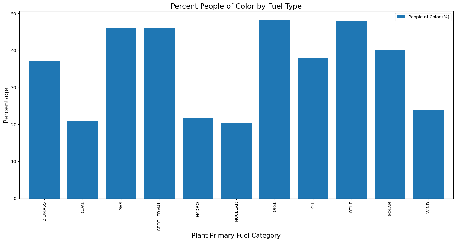
egridf.describe().Tjoined.describe().Tjoined# Create a figure with 2 rows and 3 columns
fig, axes = plt.subplots(nrows=4, ncols=2, figsize=(14, 10))
axes = axes.flatten()
cols = ['People of Color (%)', 'Low Income (%)', 'Less Than High School Education (%)', 'Limited English Speaking (%)','Unemployment Rate (%)', 'Under Age 5 (%)', 'Over Age 64 (%)']
for i, col in enumerate(cols):
ax = axes[i]
# histogram of demo % for non host communities
ax.hist(
joined[(joined['has_plant'] == 0) & (joined['EPA Region']== i+1)][col],
bins=30,
alpha=0.5,
label='Non-Host Community',
density=True
)
# histogram of demo % for host communities
ax.hist(
joined[(joined['has_plant'] == 1) & (joined['EPA Region']== i+1)][col],
bins=30,
alpha=0.6,
label='Host Community',
density=True
)
ax.set_title(f'{col}')
ax.set_xlabel(f'{col}')
ax.set_ylabel('Density')
ax.legend()
plt.suptitle('Demographic Distributions in Host vs Non-Host Communities in US Counties', fontsize = 15)
plt.tight_layout()
fig.delaxes(fig.axes[-1])
plt.show()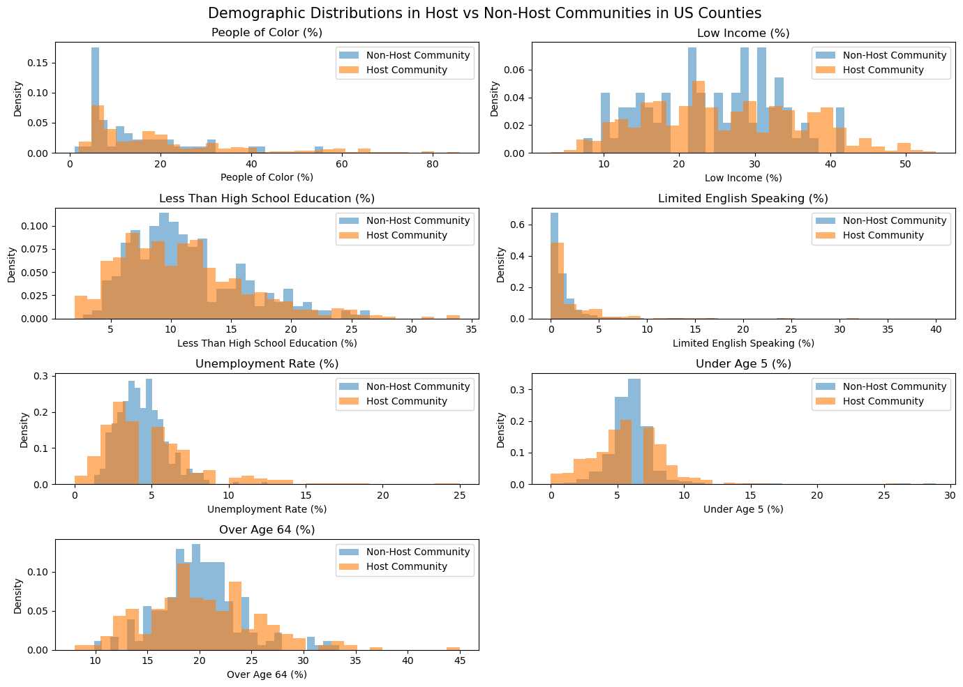
fig, axes = plt.subplots(nrows=5, ncols=2, figsize=(14, 10))
axes = axes.flatten()

#10 total regions
for i in np.arange(10):
    ax = axes[i]

    # histogram of people of color % for non host communities
    ax.hist(
        joined[(joined['has_plant'] == 0) & (joined['EPA Region']== i+1)]['People of Color (%)'],
        bins=30,
        alpha=0.5,
        label='Non-Host Community',
        density=True
    )

    # histogram of people of color % for host communities
    ax.hist(
        joined[(joined['has_plant'] == 1) & (joined['EPA Region']== i+1)]['People of Color (%)'],
        bins=30,
        alpha=0.6,
        label='Host Community',
        density=True
    )

    ax.set_title(f'EPA Region: {i+1}')
    ax.set_xlabel('People of Color (%)')
    ax.set_ylabel('Density')
    ax.legend()

plt.tight_layout()
plt.show()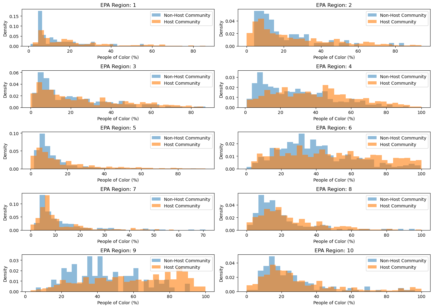
Hypothesis
Our general hypothesis is that the location of plants are disproportionately placed in marginalized communities. The characteristic of a marginalized community is not singular, which illicts the need to conduct multiple hypothesis testing to observe potential inequalities across multiple socioeconomic demographic metrics.
Our alternative hypotheses are as follows:
Plants are disproportionately located in areas with higher % People of Color
Plants are disproportionately located in areas with higher % Low Income
Plants are disproportionately located in areas with higher % Less Than High School Education
Plants are disproportionately located in areas with higher % Limited English speaking households
Plants are disproportionately located in areas with higher % Unemployment Rate
There is a difference in the percentage of people under age 5 for counties with plants vs. without
There is a difference in the percentage of people over age 64 for counties with plants vs. without
Our null hypotheses are that there is no difference in means of these demographic factors between counties with plants and counties without plants.
We will be conducting A/B testing against each hypothesis. This is because we can treat each plant in the eGRID data as the ‘treatment’ of having a plant. The other counties across the US will be the control groups, for not having a plant.
To correct for the multiple hypothesis tests, we will use two different methods:
To control the FDR at 0.05, we will use the Benjamini–Yekutieli procedure, which controls the false discovery rate under arbitrary dependence assumptions. This is needed because the demographic metrics are not independent due to the socioeconomic functioning of the US.(could add EDA on this w a correlation map)
To control for the FWER at 0.05, we will use the Bonferroni correction.
counties = pd.read_csv('data/mh_analysis_ready.csv', index_col=0)
counties# **Credit note: the functions below were based off of Reily Fairchild's homework 1 code that she developed, augmented to fit our analysis here.
def difference_of_means(df, group_label, numerical_col, abs_dif):
"""
Calculate difference in means, dependent on one or two sided test
df: dataframe
numerical_col (string): a numerical column name
binary_col (string): a binary column name that will be shuffled
i (integer): simmulation random state
abs_dif (bool): whether it is a one sided or two sided alternative hypothesis
"""
series = df.groupby('Shuffled Label').mean().loc[:, numerical_col]
if abs_dif == True:
return abs(series.iloc[1] - series.iloc[0])
else:
return series.iloc[1] - series.iloc[0]def one_simulated_difference_of_means(df, numerical_col, binary_col, i, abs_dif):
"""
The function computes a single simulation of an A/B permutation and the difference of means.
inputs
df: dataframe
numerical_col (string): a numerical column name
binary_col (string): a binary column name that will be shuffled
i (integer): simmulation random state
abs_dif (bool): whether it is a one sided or two sided alternative hypothesis
"""
shuffled_df = df.copy()
shuffled_labels = df.sample(replace=False, frac = 1, random_state = i)[binary_col]
shuf = shuffled_labels.to_numpy()
shuffled_df['Shuffled Label'] = shuf
selected_shuf = shuffled_df.loc[:, (numerical_col, 'Shuffled Label')]
return difference_of_means(selected_shuf, 'Shuffled Label', numerical_col, abs_dif)def avg_difference_in_means(df, numerical_col, abs_dif, binary_col= 'has_plant'):
"""
The function computes the p-value for a test of the following hypothesis test:
H0 : There is no difference in the average value of numerical_col between the two
groups specified in binary_col.
H1 : The average value of numerical_col is different for the two groups specified
in binary_col
inputs
numerical_col: a numerical column name
binary_col: a binary column name
"""
selected = df.loc[:, (numerical_col, binary_col)]
series_obs = selected.groupby(binary_col).mean().loc[:, numerical_col]
if abs_dif == True:
observed_difference = abs(series_obs.iloc[1] - series_obs.iloc[0])
else:
observed_difference = series_obs.iloc[1] - series_obs.iloc[0]
differences = []
repetitions = 2500
for i in np.arange(repetitions):
new_difference = one_simulated_difference_of_means(df, numerical_col, binary_col, i, abs_dif)
differences = np.append(differences, new_difference)
empirical_p = np.count_nonzero(differences >= observed_difference) / repetitions #how many samples have as extreme of a difference?
#print(f' observed dif: {observed_difference}, empirical p: {empirical_p}')
return empirical_p
one_sided_cols = ['People of Color (%)', 'Low Income (%)', 'Less Than High School Education (%)', 'Unemployment Rate (%)', 'Limited English Speaking (%)']
two_sided_cols = ['Over Age 64 (%)', 'Under Age 5 (%)']
#binary_col = 'has_plant'
pvals = {}

# one sided alternative hypothesis, namely higher %
for i in one_sided_cols:
    pvals[f'{i}'] = avg_difference_in_means(counties, i, abs_dif = True)
# two sided alternative hypothesis for ages
for k in two_sided_cols:
    pvals[f'{k}'] = avg_difference_in_means(counties, k, abs_dif = False)

pvals
{'People of Color (%)': 0.0,
'Low Income (%)': 0.0,
'Less Than High School Education (%)': 0.0064,
'Unemployment Rate (%)': 0.0,
'Limited English Speaking (%)': 0.0,
'Over Age 64 (%)': 1.0,
'Under Age 5 (%)': 0.994}Bonferroni Procedure and FWER Discoveries
fwer = 0.05
num_tests = len(one_sided_cols) + len(two_sided_cols)
fwer_threshold = fwer / num_tests
print(f'FWER threshold: {fwer_threshold}')
reject_null = [x for x in list(pvals.keys()) if pvals[x] <= fwer_threshold]

print(f'There are {len(reject_null)} discoveries made when controlling FWER are {reject_null}')
FWER threshold: 0.0071428571428571435
There are 5 discoveries made when controlling FWER are ['People of Color (%)', 'Low Income (%)', 'Less Than High School Education (%)', 'Unemployment Rate (%)', 'Limited English Speaking (%)']
Benjamini–Yekutieli Procedure and FDR Discoveries
p_sorted = sorted(list(pvals.values()))

m = len(p_sorted)
k = np.arange(1, m+1)  # index of each test in sorted order
alpha = 0.05 # desired FPR
c_m = np.sum([1/i for i in range(1, m)]) # Benjamini–Yekutieli procedure's 'harmonic function'
compare = (alpha * k) /(m * c_m) # B-y threshold
below_than = p_sorted <= compare
cols = {'k' : k, 'p-vals' : p_sorted, 'compare': compare, 'below than' : below_than}

ps = pd.DataFrame(cols)
ps
fdr_threshold = ps[ps['below than'] == True]['p-vals'].iloc[-1]
print(f'FDR threshold: {fdr_threshold}')
fdr_reject_null = [x for x in list(pvals.keys()) if pvals[x] <= fdr_threshold]
#list(pvals.values())

print(f'The are {len(fdr_reject_null)} discoveries made when controlling FDR are {fdr_reject_null}')
FDR threshold: 0.0064
The are 5 discoveries made when controlling FDR are ['People of Color (%)', 'Low Income (%)', 'Less Than High School Education (%)', 'Unemployment Rate (%)', 'Limited English Speaking (%)']
Specific Alternative Test and Likelihood Ratio Test
Null: In the United States, the distribution of People of Color % is the same for host communities as for non-host communities, on average. Simple Alternative: In the United States, host communities have 3% more People of Color, on average, than non-host communities.
The 3% was decided based on a similar study which found that communities with oil plants were 2.6% more Black, 4.2% more Latinx, and 1.4% more Asian than communities without oil plants. https://
from scipy.stats import norm
def simple_alt_hyp(df, numerical_col, binary_col= 'has_plant'):
    """
   The function computes the power for a simple alternative hypothesis test:
        H0 : There is no difference in the average value of numerical_col between the two
            groups specified in binary_col.
        H1 : The average value of numerical_col is 3%
    inputs
        df: dataframe
        numerical_col: a numerical column name
        binary_col: the treatment column name
    """
    selected = df.loc[:, (numerical_col, binary_col)]
    series_obs = selected.groupby(binary_col).mean().loc[:, numerical_col]
    observed_difference = series_obs.iloc[1] - series_obs.iloc[0]

    #calculate std of the difference between means (https://stattrek.com/sampling/difference-in-means)
    sd_treatment = (df[df[binary_col] == 1][numerical_col].std() **2) / len(df[df[binary_col] == 1][numerical_col]) #treatments var/n
    sd_control = (df[df[binary_col] == 0][numerical_col].std() **2) / len(df[df[binary_col] == 0][numerical_col]) #control var/n
    std = np.sqrt((sd_treatment) + (sd_control))

    # desired FPR
    fpr = 0.05

    # threshold = 95% quantile under the null ie any observed dif that is in the area to the right of this point will be rejected
    threshold = norm.ppf(1-fpr, loc=0, scale=std)

    #power = TPR : p( rejecting the null, given alt hypothesis is true) so p(LR > n) | x is alt
    # p( x > threshold) under the alternative
    power = 1 - norm.cdf(threshold, loc=3, scale=std)

    print(f'The observed difference is {observed_difference}, the threshold is {threshold}, and the power is: {power}')
    if observed_difference > threshold:
        print('Because the observed difference is greater than the threshold, we reject the null.')
    else:
        print('Because the observed difference is not greater than the threshold, we fail to reject the null.')
    return power
simple_alt_hyp(counties, 'People of Color (%)');The observed difference is 11.89399468701766, the threshold is 0.8235939462410474, and the power is: 0.9999930881732889
Because the observed difference is greater than the threshold, we reject the null.
RESEARCH QUESTION 2
Data Loading
Imports
import requests
from bs4 import BeautifulSoup
import io
Treatment : Price
We scrape our treatment data from Energy Information Administration website
# extract list of state codes from EIA website
url = "https://www.eia.gov/dnav/pet/pet_pri_dfp1_k_m.htm"
page = requests.get(url)
soup = BeautifulSoup(page.text, "html.parser")

exclude_codes = ["F009960", "F001236", "F003075", "F005071", "F005061", "F005074"]

codes = []
for link in soup.find_all("a"):
    href = link.get("href", "")
    text = link.text.strip()
    if "s=F" in href and "&f=M" in href:
        code = href.split("s=")[-1].split("&")[0]
        num_part = int(code[1:7])
        if num_part % 1000 == 0:
          continue
        if code[:7] in exclude_codes:
          continue
        codes.append(code)
display(codes)
['F001242__3',
'F001354__3',
'F002017__3',
'F002018__3',
'F002020__3',
'F002021__3',
'F002026__3',
'F002031__3',
'F002038__3',
'F002039__3',
'F002040__3',
'F002046__3',
'F003001__3',
'F003005__3',
'F003022__3',
'F003028__3',
'F003035__3',
'F003048__3',
'F004008__3',
'F004030__3',
'F004049__3',
'F004056__3',
'F005006__3']all_data = []
API_URL = "https://api.eia.gov/v2/petroleum/pri/dfp1/data/"
# call the EIA API
for code in codes:
params = {
"api_key": "vUc8dcxSykilX0CpePaERE6F0NRipDBTqiB1Jl51",
"frequency": "monthly",
"data[0]": "value",
"facets[series][]": code,
"sort[0][column]": "period",
"sort[0][direction]": "desc",
"offset": 0,
"length": 5000
}
try:
response = requests.get(API_URL, params=params)
response.raise_for_status()
data = response.json()
# Extract records
for r in data['response']['data']:
all_data.append({
"State_Code": code,
"Period": r['period'],
"Price": r['value']
})
except Exception as e:
print(f"Error fetching data for code {code}: {e}")
# Convert to DataFrame and convert dates to appropriate format
df = pd.DataFrame(all_data)
df['Period'] = pd.to_datetime(df['Period'])
df['Year'] = df['Period'].dt.year
df['Month'] = df['Period'].dt.month
df = df[(df['Year'] >= 1978) & (df['Year'] <= 2024)]
df.sort_values(by=['State_Code', 'Year', 'Month'], inplace=True)
df.head()# data cleaning: remove rows where price is withdrawn
df['Price'] = pd.to_numeric(df['Price'], errors='coerce')
df = df.dropna(subset=['Price'])
df = df.reset_index(drop=True)# add state column
state_mapping = {
'F001242__3': 'PA',
'F001354__3': 'WV',
'F002017__3': 'IL',
'F002018__3': 'IN',
'F002020__3': 'KS',
'F002021__3': 'KY',
'F002026__3': 'MI',
'F002031__3': 'NE',
'F002038__3': 'ND',
'F002039__3': 'OH',
'F002040__3': 'OK',
'F002046__3': 'SD',
'F003001__3': 'AL',
'F003005__3': 'AR',
'F003022__3': 'LA',
'F003028__3': 'MS',
'F003035__3': 'NM',
'F003048__3': 'TX',
'F004008__3': 'CO',
'F004030__3': 'MT',
'F004049__3': 'UT',
'F004056__3': 'WY',
'F005006__3': 'CA'
}
# get state mappings
df['state'] = df['State_Code'].map(state_mapping)
print(df.head(10))
print(df.shape) State_Code Period Price Year Month state
0 F001242__3 1978-01-01 14.71 1978 1 PA
1 F001242__3 1978-02-01 14.80 1978 2 PA
2 F001242__3 1978-03-01 14.74 1978 3 PA
3 F001242__3 1978-04-01 14.67 1978 4 PA
4 F001242__3 1978-05-01 14.71 1978 5 PA
5 F001242__3 1978-06-01 14.72 1978 6 PA
6 F001242__3 1978-07-01 14.75 1978 7 PA
7 F001242__3 1978-08-01 14.65 1978 8 PA
8 F001242__3 1978-09-01 14.70 1978 9 PA
9 F001242__3 1978-10-01 14.78 1978 10 PA
(12784, 6)
Outcome : Consumption
We join our outcome variable data from external data source: https://
cons_csv = pd.read_csv('data/consumption_data.csv')
cons_csv.head(20)# filter for only petroleum derived electricity consumption
cons_csv = cons_csv[(cons_csv['ENERGY SOURCE (UNITS)'].str.contains('Petroleum')) & (cons_csv['TYPE OF PRODUCER']=='Total Electric Power Industry')]
print(cons_csv.head())
print(cons_csv.shape) YEAR MONTH STATE TYPE OF PRODUCER \
1 2001 1 AK Total Electric Power Industry
13 2001 1 AL Total Electric Power Industry
29 2001 1 AR Total Electric Power Industry
39 2001 1 AZ Total Electric Power Industry
51 2001 1 CA Total Electric Power Industry
ENERGY SOURCE (UNITS) CONSUMPTION
1 Petroleum (Barrels) 124,998
13 Petroleum (Barrels) 284,241
29 Petroleum (Barrels) 209,194
39 Petroleum (Barrels) 268,016
51 Petroleum (Barrels) 960,824
(15392, 6)
# join the two tables
cons_csv['YEAR'] = cons_csv['YEAR'].astype('int32')
cons_csv['MONTH'] = cons_csv['MONTH'].astype('int32')
df = df.merge(cons_csv, left_on=['Year', 'state', 'Month'], right_on=['YEAR', 'STATE', 'MONTH'], how='inner')
df = df.drop(columns=['YEAR', 'STATE', 'MONTH'])

# data cleaning : set to numeric
df['CONSUMPTION'] = pd.to_numeric(
    df['CONSUMPTION'].astype(str).str.replace(',', ''),
    errors='coerce'
).astype(pd.Int64Dtype())
print(df.head())
print(df.shape)
State_Code Period Price Year Month state \
0 F001242__3 2001-01-01 28.02 2001 1 PA
1 F001242__3 2001-02-01 28.52 2001 2 PA
2 F001242__3 2001-03-01 26.20 2001 3 PA
3 F001242__3 2001-04-01 26.31 2001 4 PA
4 F001242__3 2001-05-01 27.43 2001 5 PA
TYPE OF PRODUCER ENERGY SOURCE (UNITS) \
0 Total Electric Power Industry Petroleum (Barrels)
1 Total Electric Power Industry Petroleum (Barrels)
2 Total Electric Power Industry Petroleum (Barrels)
3 Total Electric Power Industry Petroleum (Barrels)
4 Total Electric Power Industry Petroleum (Barrels)
CONSUMPTION
0 1005652
1 196117
2 478840
3 960097
4 524322
(6499, 9)
Yield
Join confounder yield curve data from external source: https://
yield_curve = pd.read_csv('data/treasury_data.csv')
yield_curve.head()# join with existing df
yield_curve.rename(columns={'T10Y2YM':'Treasury Yield Spread (10Y-2Y)'}, inplace=True)
yield_curve['Year'] = yield_curve['observation_date'].str.split('-').str[0]
yield_curve['Month'] = yield_curve['observation_date'].str.split('-').str[1]
yield_curve.drop(columns=['observation_date'], inplace=True)
yield_curve['Year'] = yield_curve['Year'].astype('int32')
yield_curve['Month'] = yield_curve['Month'].astype('int32')
yield_curve.drop_duplicates(subset=['Year', 'Month'], keep='first', inplace=True)
df = df.merge(yield_curve, on=['Year','Month'], how='inner')
print(df.head())
print(df.shape) State_Code Period Price Year Month state \
0 F001242__3 2001-01-01 28.02 2001 1 PA
1 F001242__3 2001-02-01 28.52 2001 2 PA
2 F001242__3 2001-03-01 26.20 2001 3 PA
3 F001242__3 2001-04-01 26.31 2001 4 PA
4 F001242__3 2001-05-01 27.43 2001 5 PA
TYPE OF PRODUCER ENERGY SOURCE (UNITS) \
0 Total Electric Power Industry Petroleum (Barrels)
1 Total Electric Power Industry Petroleum (Barrels)
2 Total Electric Power Industry Petroleum (Barrels)
3 Total Electric Power Industry Petroleum (Barrels)
4 Total Electric Power Industry Petroleum (Barrels)
CONSUMPTION T10Y2Y
0 1005652 NaN
1 196117 0.55
2 478840 0.46
3 960097 0.76
4 524322 1.07
(6499, 10)
Inflation
Join confounder inflation rate data from external source: https://
inflation = pd.read_csv('data/inflation_data.csv')
inflation.head()# join with existing df
inflation.rename(columns={'FPCPITOTLZGUSA':'Inflation Rate (%)'}, inplace=True)
inflation['Year'] = inflation['observation_date'].str.split('-').str[0]
inflation.drop(columns=['observation_date'], inplace=True)
inflation['Year'] = inflation['Year'].astype('int32')
df = df.merge(inflation, on='Year', how='inner')
print(df.head())
print(df.shape) State_Code Period Price Year Month state \
0 F001242__3 2001-01-01 28.02 2001 1 PA
1 F001242__3 2001-02-01 28.52 2001 2 PA
2 F001242__3 2001-03-01 26.20 2001 3 PA
3 F001242__3 2001-04-01 26.31 2001 4 PA
4 F001242__3 2001-05-01 27.43 2001 5 PA
TYPE OF PRODUCER ENERGY SOURCE (UNITS) \
0 Total Electric Power Industry Petroleum (Barrels)
1 Total Electric Power Industry Petroleum (Barrels)
2 Total Electric Power Industry Petroleum (Barrels)
3 Total Electric Power Industry Petroleum (Barrels)
4 Total Electric Power Industry Petroleum (Barrels)
CONSUMPTION T10Y2Y Inflation Rate (%)
0 1005652 NaN 2.826171
1 196117 0.55 2.826171
2 478840 0.46 2.826171
3 960097 0.76 2.826171
4 524322 1.07 2.826171
(6499, 11)
Industrial Production Index
Join confounder industrial production index data from external source: https://
ind_idx = pd.read_csv('data/industrial_production_data.csv')
ind_idx.head()# join with existing df
ind_idx.rename(columns={'INDPRO':'Industrial Production Index'}, inplace=True)
ind_idx['Year'] = ind_idx['observation_date'].str.split('-').str[0]
ind_idx['Month'] = ind_idx['observation_date'].str.split('-').str[1]
ind_idx.drop(columns=['observation_date'], inplace=True)
ind_idx['Year'] = ind_idx['Year'].astype('int32')
ind_idx['Month'] = ind_idx['Month'].astype('int32')
df = df.merge(ind_idx, on=['Year', 'Month'], how='inner')
print(df.head())
print(df.shape) State_Code Period Price Year Month state \
0 F001242__3 2001-01-01 28.02 2001 1 PA
1 F001242__3 2001-02-01 28.52 2001 2 PA
2 F001242__3 2001-03-01 26.20 2001 3 PA
3 F001242__3 2001-04-01 26.31 2001 4 PA
4 F001242__3 2001-05-01 27.43 2001 5 PA
TYPE OF PRODUCER ENERGY SOURCE (UNITS) \
0 Total Electric Power Industry Petroleum (Barrels)
1 Total Electric Power Industry Petroleum (Barrels)
2 Total Electric Power Industry Petroleum (Barrels)
3 Total Electric Power Industry Petroleum (Barrels)
4 Total Electric Power Industry Petroleum (Barrels)
CONSUMPTION T10Y2Y Inflation Rate (%) Industrial Production Index
0 1005652 NaN 2.826171 91.9020
1 196117 0.55 2.826171 91.3034
2 478840 0.46 2.826171 91.1162
3 960097 0.76 2.826171 90.7891
4 524322 1.07 2.826171 90.3555
(6499, 12)
Weather
Join confounder weather data by calling NOAA API
# integrate temperature on monthly state-level basis
import time

# call NOAA endpoint to extract weather data
noaa_url = "https://www.ncei.noaa.gov/access/monitoring/climate-at-a-glance/statewide/time-series/{state}/tavg/1/0/2000-2025.json"
all_data = []

for state_id in range(1, 51):
    url = noaa_url.format(state=state_id)
    try:
        r = requests.get(url, timeout=10)
        r.raise_for_status()
        j = r.json()
        for date, value in j["data"].items():
            year = int(date[:4])
            month = int(date[4:])
            all_data.append({
                "state_id": state_id,
                "year": year,
                "month": month,
                "temperature": value
            })

    except Exception as e:
        print(f"State {state_id} failed: {e}")

    time.sleep(0.4)

tmp = pd.DataFrame(all_data)
print(tmp.head())
print(tmp.shape)
State 49 failed: 404 Client Error: Not Found for url: https://www.ncei.noaa.gov/access/monitoring/climate-at-a-glance/statewide/time-series/49/tavg/1/0/2000-2025.json
state_id year month temperature
0 1 2000 1 {'value': 46.5}
1 1 2000 2 {'value': 52.3}
2 1 2000 3 {'value': 58.9}
3 1 2000 4 {'value': 60.1}
4 1 2000 5 {'value': 74}
(15239, 4)
def extract_temp(val):
  return val['value']

tmp['temperature'] = tmp['temperature'].apply(extract_temp)

state_id_to_code = {
    1: "AL", 2: "AZ", 3: "AR", 4: "CA", 5: "CO",
    6: "CT", 7: "DE", 8: "FL", 9: "GA", 10: "HI",
    11: "ID", 12: "IL", 13: "IN", 14: "IA", 15: "KS",
    16: "KY", 17: "LA", 18: "ME", 19: "MD", 20: "MA",
    21: "MI", 22: "MN", 23: "MS", 24: "MO", 25: "MT",
    26: "NE", 27: "NV", 28: "NH", 29: "NJ", 30: "NM",
    31: "NY", 32: "NC", 33: "ND", 34: "OH", 35: "OK",
    36: "OR", 37: "PA", 38: "RI", 39: "SC", 40: "SD",
    41: "TN", 42: "TX", 43: "UT", 44: "VT", 45: "VA",
    46: "WA", 47: "WV", 48: "WI", 49: "WY", 50: "AK"
}

# map code to existing state abbrev
tmp['State'] = tmp['state_id'].map(state_id_to_code)
tmp.drop(columns=['state_id'], inplace=True)
tmp.head()# merge with existing df
tmp.rename(columns={'temperature':'temperature (F)','year':'Year','month':'Month','State':'state'}, inplace=True)
tmp['Year'] = tmp['Year'].astype('int32')
tmp['Month'] = tmp['Month'].astype('int32')
df = df.merge(tmp, on=['state', 'Year', 'Month'], how='inner')
print(df.head())
print(df.shape) State_Code Period Price Year Month state \
0 F001242__3 2001-01-01 28.02 2001 1 PA
1 F001242__3 2001-02-01 28.52 2001 2 PA
2 F001242__3 2001-03-01 26.20 2001 3 PA
3 F001242__3 2001-04-01 26.31 2001 4 PA
4 F001242__3 2001-05-01 27.43 2001 5 PA
TYPE OF PRODUCER ENERGY SOURCE (UNITS) \
0 Total Electric Power Industry Petroleum (Barrels)
1 Total Electric Power Industry Petroleum (Barrels)
2 Total Electric Power Industry Petroleum (Barrels)
3 Total Electric Power Industry Petroleum (Barrels)
4 Total Electric Power Industry Petroleum (Barrels)
CONSUMPTION T10Y2Y Inflation Rate (%) Industrial Production Index \
0 1005652 NaN 2.826171 91.9020
1 196117 0.55 2.826171 91.3034
2 478840 0.46 2.826171 91.1162
3 960097 0.76 2.826171 90.7891
4 524322 1.07 2.826171 90.3555
temperature (F)
0 28.0
1 30.9
2 35.3
3 47.5
4 58.9
(6211, 13)
Electricity Price
Join confounder electricity price data from external source: https://
prices = pd.read_csv('data/electricity_price_data.csv')
prices.head()# remove empty columns
remove_colums = []
for col in prices.columns:
if 'Unnamed' in col:
remove_colums.append(col)
prices.drop(columns=remove_colums, inplace=True)
prices = prices.melt(
id_vars=["State"], # Columns to keep
var_name="Year", # Name for the new "variable" column
value_name="Price" # Name for the new "value" column
)
# Convert Year and Price to numeric
prices["Year"] = prices["Year"].astype(int)
prices["Price"] = pd.to_numeric(prices["Price"], errors='coerce')
print(prices.head()) State Year Price
0 AK 1970 1.39
1 AL 1970 1.37
2 AR 1970 1.51
3 AZ 1970 1.97
4 CA 1970 1.74
# join with existing df
prices.rename(columns={'Price':'Electricity Price ($ per million BTU)','State':'state'}, inplace=True)
prices['Year'] = prices['Year'].astype('int32')
df = df.merge(prices, on=['state', 'Year'], how='inner')
print(df.head())
print(df.shape)
State_Code Period Price Year Month state \
0 F001242__3 2001-01-01 28.02 2001 1 PA
1 F001242__3 2001-02-01 28.52 2001 2 PA
2 F001242__3 2001-03-01 26.20 2001 3 PA
3 F001242__3 2001-04-01 26.31 2001 4 PA
4 F001242__3 2001-05-01 27.43 2001 5 PA
TYPE OF PRODUCER ENERGY SOURCE (UNITS) \
0 Total Electric Power Industry Petroleum (Barrels)
1 Total Electric Power Industry Petroleum (Barrels)
2 Total Electric Power Industry Petroleum (Barrels)
3 Total Electric Power Industry Petroleum (Barrels)
4 Total Electric Power Industry Petroleum (Barrels)
CONSUMPTION T10Y2Y Inflation Rate (%) Industrial Production Index \
0 1005652 NaN 2.826171 91.9020
1 196117 0.55 2.826171 91.3034
2 478840 0.46 2.826171 91.1162
3 960097 0.76 2.826171 90.7891
4 524322 1.07 2.826171 90.3555
temperature (F) Electricity Price ($ per million BTU)
0 28.0 11.26
1 30.9 11.26
2 35.3 11.26
3 47.5 11.26
4 58.9 11.26
(5947, 14)
OPEC Supply
Join confounder OPEC supply data
opec = pd.read_csv('data/OPEC_data.csv')
opec.head()# extract years as distinct rows
opec = pd.melt(opec, var_name='Year', value_name='OPEC supply (1000 b/d)')
opec.head()opec['Year'] = opec['Year'].astype(int)
df = df.merge(opec, on='Year')
# data cleaning : set to numeric
df['OPEC supply (1000 b/d)'] = pd.to_numeric(
df['OPEC supply (1000 b/d)'].astype(str).str.replace(',', ''),
errors='coerce'
).astype(pd.Int64Dtype())
df.head()# save aggregated data
df.to_csv('data/data102_oil_data_final.csv')RQ2: Generating Visualizations for EDA
# visualize treatment vs outcome
plt.figure(figsize=(10, 6))
plt.scatter(df['Price'], df['CONSUMPTION'], alpha=0.1)
plt.xlabel('Price ($/barrel)')
plt.ylabel('Consumption (barrels)')
plt.title('Oil Price vs. Petroleum-derived Electricity Consumption')
plt.grid(True)
plt.tight_layout()
plt.show()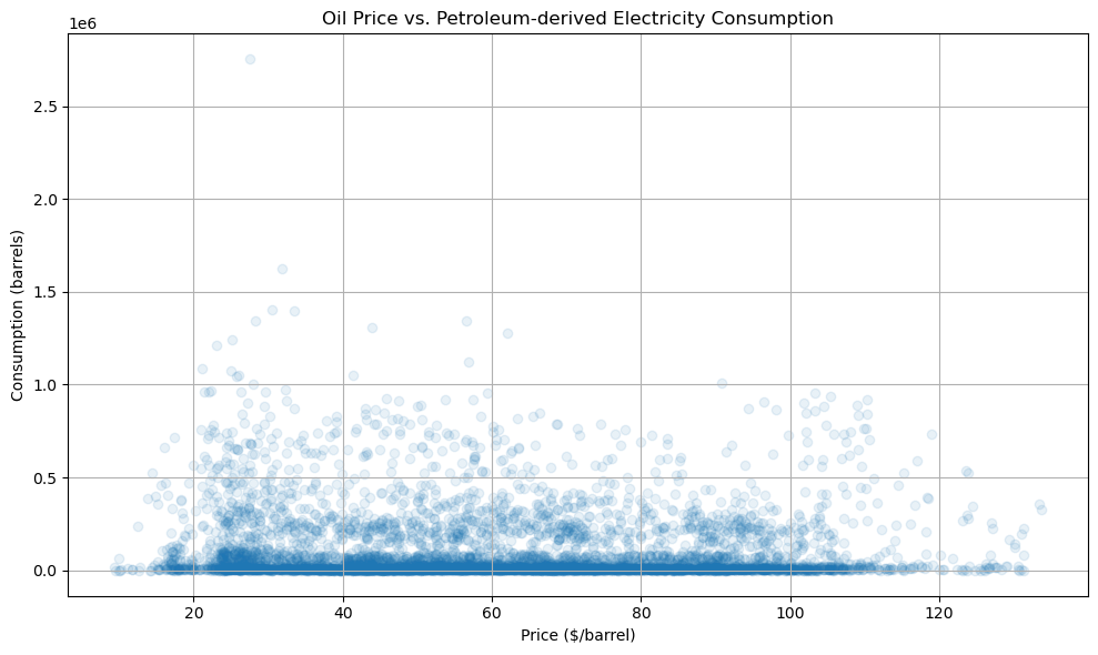
# visualize treatment - outcome correlations state by state
state_vals = df['state'].unique()
corr_vals = []
for curr_val in state_vals:
  curr_df = df[df['state'] == curr_val]
  corr_vals.append(curr_df['Price'].corr(curr_df['CONSUMPTION']))

plt.hist(corr_vals, bins=10)
plt.xlabel('Correlation Value')
plt.ylabel('Frequency')
plt.title('Histogram of Treatement-Target Correlation Values by State')
plt.show()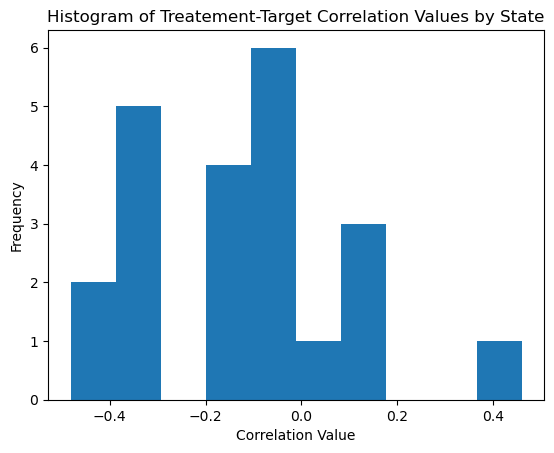
# visualize confounder - outcome relationships
target = 'CONSUMPTION'
exclude_features = ['Period', 'Year', 'Month', 'CONSUMPTION', 'state', 'State_Code']
features = [col for col in df.columns if col not in exclude_features]
features = features[-6:]

nrows, ncols = 3, 2
fig, axes = plt.subplots(nrows=nrows, ncols=ncols, figsize=(15, 12))
axes = axes.flatten()

num_plots = len(features)

for i in range(num_plots):
    feature = features[i]
    ax = axes[i]

    sns.scatterplot(x=df[feature], y=df[target], alpha=0.4, ax=ax)

    ax.set_title(f'{feature} vs. Consumption', fontsize=14)
    ax.set_xlabel(feature, fontsize=12)
    ax.set_ylabel('Consumption (barrels)', fontsize=12)

for j in range(num_plots, nrows * ncols):
    if j < len(axes):
        fig.delaxes(axes[j])

plt.tight_layout()
plt.show()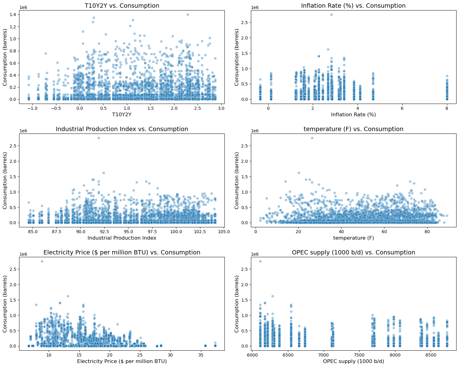
Modeling
Feature Engineering
# one hot encode state column
df = pd.get_dummies(df, columns=['state'], dtype=int)
df.head()for col in df.columns:
print(f"column: {col}, type: {type(df[col].iloc[0])}")column: State_Code, type: <class 'str'>
column: Period, type: <class 'pandas._libs.tslibs.timestamps.Timestamp'>
column: Price, type: <class 'numpy.float64'>
column: Year, type: <class 'numpy.int32'>
column: Month, type: <class 'numpy.int32'>
column: TYPE OF PRODUCER, type: <class 'str'>
column: ENERGY SOURCE (UNITS), type: <class 'str'>
column: CONSUMPTION, type: <class 'numpy.int64'>
column: T10Y2Y, type: <class 'numpy.float64'>
column: Inflation Rate (%), type: <class 'numpy.float64'>
column: Industrial Production Index, type: <class 'numpy.float64'>
column: temperature (F), type: <class 'numpy.float64'>
column: Electricity Price ($ per million BTU), type: <class 'numpy.float64'>
column: OPEC supply (1000 b/d), type: <class 'numpy.int64'>
column: state_AL, type: <class 'numpy.int64'>
column: state_AR, type: <class 'numpy.int64'>
column: state_CA, type: <class 'numpy.int64'>
column: state_CO, type: <class 'numpy.int64'>
column: state_IL, type: <class 'numpy.int64'>
column: state_IN, type: <class 'numpy.int64'>
column: state_KS, type: <class 'numpy.int64'>
column: state_KY, type: <class 'numpy.int64'>
column: state_LA, type: <class 'numpy.int64'>
column: state_MI, type: <class 'numpy.int64'>
column: state_MS, type: <class 'numpy.int64'>
column: state_MT, type: <class 'numpy.int64'>
column: state_ND, type: <class 'numpy.int64'>
column: state_NE, type: <class 'numpy.int64'>
column: state_NM, type: <class 'numpy.int64'>
column: state_OH, type: <class 'numpy.int64'>
column: state_OK, type: <class 'numpy.int64'>
column: state_PA, type: <class 'numpy.int64'>
column: state_SD, type: <class 'numpy.int64'>
column: state_TX, type: <class 'numpy.int64'>
column: state_UT, type: <class 'numpy.int64'>
column: state_WV, type: <class 'numpy.int64'>
# apply seasonality feature
model_df = df.copy()
model_df['time_idx'] = (model_df['Year'] - 2000) * 12 + (model_df['Month'] - 1)
model_df['month_sin'] = np.sin(2 * np.pi * model_df['Month'] / 12)
model_df['month_cos'] = np.cos(2 * np.pi * model_df['Month'] / 12)
model_df.rename(columns={'ENERGY SOURCE              (UNITS)': 'ENERGY SOURCE (UNITS)'}, inplace=True)

# Set to ordered format
model_df['Period'] = pd.to_datetime(model_df['Period'])

model_df.drop(columns=['State_Code', 'TYPE OF PRODUCER', 'ENERGY SOURCE (UNITS)'], inplace=True)
print(model_df.info())
<class 'pandas.core.frame.DataFrame'>
RangeIndex: 5947 entries, 0 to 5946
Data columns (total 36 columns):
# Column Non-Null Count Dtype
--- ------ -------------- -----
0 Period 5947 non-null datetime64[ns]
1 Price 5947 non-null float64
2 Year 5947 non-null int32
3 Month 5947 non-null int32
4 CONSUMPTION 5947 non-null Int64
5 T10Y2Y 5302 non-null float64
6 Inflation Rate (%) 5947 non-null float64
7 Industrial Production Index 5947 non-null float64
8 temperature (F) 5947 non-null float64
9 Electricity Price ($ per million BTU) 5947 non-null float64
10 OPEC supply (1000 b/d) 5947 non-null Int64
11 state_AL 5947 non-null int64
12 state_AR 5947 non-null int64
13 state_CA 5947 non-null int64
14 state_CO 5947 non-null int64
15 state_IL 5947 non-null int64
16 state_IN 5947 non-null int64
17 state_KS 5947 non-null int64
18 state_KY 5947 non-null int64
19 state_LA 5947 non-null int64
20 state_MI 5947 non-null int64
21 state_MS 5947 non-null int64
22 state_MT 5947 non-null int64
23 state_ND 5947 non-null int64
24 state_NE 5947 non-null int64
25 state_NM 5947 non-null int64
26 state_OH 5947 non-null int64
27 state_OK 5947 non-null int64
28 state_PA 5947 non-null int64
29 state_SD 5947 non-null int64
30 state_TX 5947 non-null int64
31 state_UT 5947 non-null int64
32 state_WV 5947 non-null int64
33 time_idx 5947 non-null int32
34 month_sin 5947 non-null float64
35 month_cos 5947 non-null float64
dtypes: Int64(2), datetime64[ns](1), float64(8), int32(3), int64(22)
memory usage: 1.6 MB
None
Estimate ATE using Horvitz–Thompson formula
from sklearn.model_selection import train_test_split
import statsmodels.api as sm
# remove NaN values from dataset
model_df.dropna(inplace=True)random_state=42
treatment = 'Price'
outcome = 'CONSUMPTION'
ate_df = model_df.copy()
treatment_med = ate_df['Price'].median()
T = np.where(ate_df['Price'] >= treatment_med, 1, 0).astype(np.int32)
ate_df.drop(columns=['Period', 'Year', 'Month'], errors='ignore', inplace=True)
features = [col for col in ate_df.columns if col not in ['CONSUMPTION', 'Price']]
X_confounders = ate_df[features]
X_array = X_confounders.values.astype(float)
X_confounders_sm = sm.add_constant(X_array, prepend=True)
T_array = T.astype(float)
# Run the Logit model
logit_model = sm.Logit(T_array, X_confounders_sm)
logit_results = logit_model.fit(disp=0)
# Calculate propensity scores
propensity_scores = logit_results.predict(X_confounders_sm)
ate_df['propensity_score'] = propensity_scores
ate_df['T'] = T
# Perform Trimming on Extreme Propensity Values
lower, upper = 0.025, 0.975
mask = (
(ate_df['propensity_score'] > lower) &
(ate_df['propensity_score'] < upper)
)
ate_trim = ate_df.loc[mask].copy()
Y = ate_trim[outcome].values
T_trim = ate_trim['T'].values
e = ate_trim['propensity_score'].values
N = len(ate_trim)
# Horvitz–Thompson IPW ATE formula: Sum[ (T*Y/e) - ((1-T)*Y/(1-e)) ] / N
ate_ht = (1 / N) * np.sum(
(T_trim * Y / e) - ((1 - T_trim) * Y / (1 - e))
)
print(f"Horvitz–Thompson IPW ATE (HT): {ate_ht:.4f}")Horvitz–Thompson IPW ATE (HT): -6915.6903
According to our findings, a $1 increase in price causes, on average, a decrease of about 6,916 barrels of oil consumption.